3 Tips In Finding Data Easily In Google Spreadsheets

Google sheets are more than just a spreadsheet. They’re actually online and offline software that lets you do so much. From recording simple data to creating a dashboard for your marketing efforts, Google sheets offer an easy and accessible way to do such things. Especially if you’re engaged in business or in the blogging industry, you can use Google sheets as a convenient record-keeping tool.
As you can save your data in your Google Drive, you can open it anytime and anywhere. Since it has become a vital tool for so many people, you might also be using it to record a lot of data. When this happens, you may find it hard to manually search for the information that you need.
That’s why here are some tips you can use to find data in your Google sheets without too much hardship:
Table of contents
1. Use LOOKUP Functions
One of the many things you can do with Google spreadsheets is to enter data with the sums and values of each piece of information. For instance, you can list down the title of blogs you post, who the writers are, and where they’re posted. Great, right? But what if you need to sort things out by a certain category in the author sheet?
Like for example, you want to know the number of blogs your writer produces and their title. Well, here’s a way of finding such data without manually sifting through your spreadsheet:
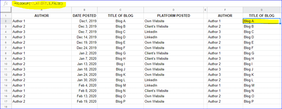
- VLOOKUP Function – when you’re using vlookup in Google sheets, you can find data from the same or multiple sheets for the closest or exact matches. For instance, if you want to sort out the title and author from your general list of blogs, you can do so. You can use the formula “=VLOOKUP (Search_Key, Range, Index, Is_Sorted)”, wherein the value of the “search_key” is what you’re actually trying to sort. The “range” refers to the cell range of the data you’re looking for, like A1 to D17, while the “index” is the number of columns of the range chosen to search for your data. Lastly, the “is_sorted” refers to the closest or exact match of your search key value.
Using the example below, you can use this VLOOKUP formula “=VLOOKUP(A2,A1:D17,3,FALSE)” if you want the author and their contributions only.
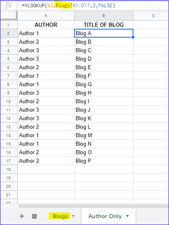
Or, if you want to use another sheet of the same spreadsheet, add the title of the sheet before the range. Your VLOOKUP formula will look like the one shown below: “=VLOOKUP(A2,Blogs!A1:D17,3,FALSE)”.
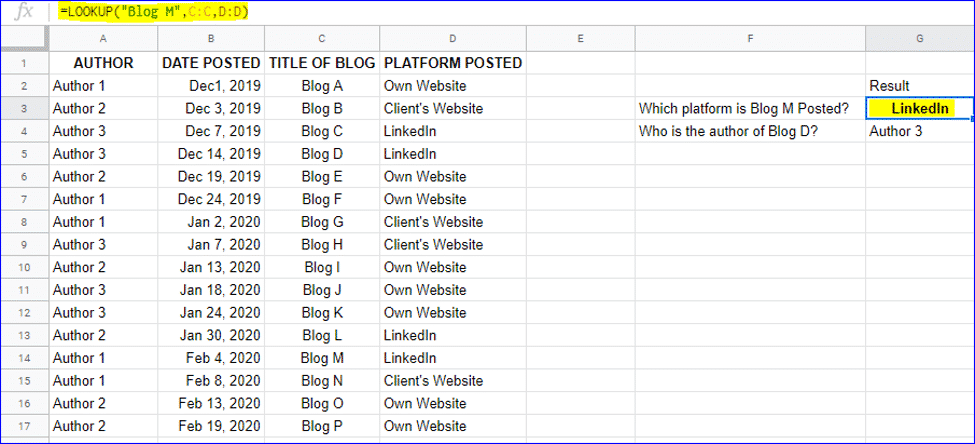
- LOOKUP Formula – Similar to VLOOKUP, the LOOKUP formula finds data from a column or row. In this function, you should have sorted the row or column for it to work. The formula is written as “LOOKUP(search_key, search_range|search_result_array, [result_range])”, wherein the “search_key” refers to the value that the function is meant to search for. When the “search_range” finds data from the first column or row, then the value appears in the last column or row of the array, and the “result_range” then refers to the cell range where the result shows up. In short, “result_range” corresponds to the matched value of the “search_range”.
Using the same example above, if you want to know on which platform “Blog M” has been posted, then use the formula “=LOOKUP(“Blog M”,C:C,D:D)” as shown below:
- HLOOKUP Formula – this function works horizontally or finds data in the rows of a range. The formula you can use is “=HLOOKUP(search_key, range, index, [is_sorted])”. This is similar to VLOOKUP, but you can use this function if your data or record are horizontally arranged.
Using the example above but in a horizontal setting, here’s the formula you can use to know when Author 3 posted Blog C: “=HLOOKUP(“Author 3”,A1:D4,2,FALSE)”.
-
Add Links
Another way to make your life easier with Google sheets is by adding a hyperlink that you can then just click on. A link can save you time in looking for data, especially when you’ve got vast amounts of data in every sheet or spreadsheet. Or, if you’re forgetful, a link can save you the trouble of straining your brain trying to remember where the data is stored.
For instance, if you’ve got too much information in one spreadsheet, making a table of contents that displays on which sheet a record is located is highly recommended. Say you’ve got hundreds of ghostwriters working for your linking services, then creating a list of their names or usernames will save you several minutes of browsing through the spreadsheet.
Then, you should add the hyperlink to the sheet where the writer’s records are located. That way, if you need to check on each writer’s data, just click on the name on the list, and it’ll automatically lead you to the writer’s sheet.
Not only that, but you can use hyperlinks to send you to a URL related to a cell’s data. For instance, you can simply link to the blog title’s URL, so that you can go to the blog without having to search for it in the search engines.
3. Utilize the Find And Replace Button
If you’re searching for data on one sheet only, there’s a simple way of doing it, too. However, this way is only practical if you know the keywords you’re looking for. Or if you want to replace a piece of data, but you need to do it for all the relevant bits of data, you can also use the “Find and Replace” function of google sheets.
For instance, if you’re assigning a new name for existing data, then you can change all the existing data in one go. No more manually finding the data that you want to change.
If you’re in the business industry and you want to change “Tea” to “Herbal Tea,” then all you need is to press CTRL+H. The “Find and Replace” function will appear immediately so you can type in the word “Tea” in the Find bar, and type in “Herbal Tea” in the Replace bar to complete the task.
What’s more convenient is that the “Find and Replace” function gives you the option to search in all the sheets of the spreadsheet, a specific range, or just the particular sheet you’re in. Then you can also choose whether to replace every searched “Tea” or just change a specific cell.
With such a function, you can easily edit or replace a word or data without missing even a single one.
Conclusion:
Don’t be afraid to use Google spreadsheets, whether for personal or work-related purposes. You won’t get lost navigating each sheet as there are ways to make the most out of your Google sheets. One of these aspects is finding data within your sheet or spreadsheet without spending too much time searching. With the given formulas, you can use them to look for an answer on your sheet, especially if you have a massive volume of entries.
On the other hand, before looking up any data, you can add hyperlinks for easier navigation throughout your spreadsheet or even outside it. Furthermore, if you need to do some replacements of specific data, you can also do it via Google sheets’ “Find and Replace” function.
